
Introduction
In a previous article, we saw that measuring shutter speed presents no particular difficulty at low speeds, but that things become much more challenging at high speeds.
We also saw that two methods can be considered for measuring shutter speed:
- Timer-based measurement
- Integration-based measurement
Based on abstract shutter opening curves, we examined the consequences of these two methods in terms of measurement reliability.
In this second part, I propose:
- identifying the two main shutter families;
- studying how leaf shutters work and how their operation affects the opening profile;
- studying, using real measurements, how the measurement method affects the reliability of the result.
Two Shutter Families
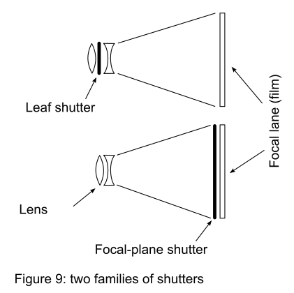
Shutters can be divided into two distinct families: leaf shutters and focal-plane shutters.
- A leaf shutter is located close to the optical center, generally inside the lens.
- A focal-plane shutter is located close to the focal plane, i.e. close to the film or image sensor.
Leaf shutters
Leaf shutters are found mainly at the two extremes of the camera-format spectrum:
- medium- and large-format cameras;
- compact cameras.
Their advantages include:
- simultaneous illumination of the entire image;
- flash synchronization over the entire shutter-speed range, as a consequence of the previous point;
- relatively low manufacturing cost when they are small and have modest performance requirements, as is the case with compact cameras.
Their disadvantages include:
- imited maximum shutter speeds, most commonly 1/250 s or 1/500 s, especially when the aperture is large;
- when integrated into the lens, they increase the cost of the lens.
Focal-Plane Shutters
Focal-plane shutters are found mainly in 35 mm cameras, both SLR and rangefinder cameras.
Their advantages include:
- very high shutter speeds, typically 1/1000 s or faster;
- being integrated into the camera body, so there is no additional shutter cost for each lens.
Their disadvantages include:
- the entire image is not exposed simultaneously;
- a limited X-sync speed, as a consequence of the previous point;
- relatively high manufacturing costs, and the fact that they are delicate to adjust and service.
Focal-plane shutters will be examined in detail in future articles.
Leaf Shutter: Operating Principle and Measurement Setup
As mentioned above, a leaf shutter is located close to the optical center of the camera. It is also called a leaf shutter in English because it is often made of blades that open and close to let light through or block it.
Its speed is limited by the mechanical inertia of the blades, which have to open and close across the entire shutter aperture.
A leaf shutter allows the entire image to be illuminated simultaneously. However, the illumination is progressive. Since every part of the shutter contributes to illuminating every point of the image, as a consequence of the imaging properties of the lens, the illuminance increases progressively as the shutter opens and decreases progressively as it closes.
To correctly account for this behavior and reproduce real operating conditions as closely as possible, a leaf shutter must therefore be tested using a diffuse light source illuminating its entire surface, so that the whole shutter aperture is taken into account.
Furthermore, in order to take the entire shutter surface into account, the test must be performed with the lens wide open.
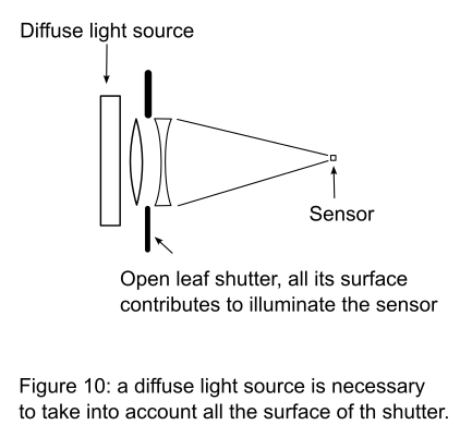
It should be noted that if the light source is diffuse and relatively close to the shutter, every point of the focal plane is illuminated equally, apart from vignetting. The measured illuminance curve therefore does not depend on the size of the sensor.
Experimental Curves and Interpretation
The experimental curves presented in this article were recorded using a digital oscilloscope connected to a Baby Shutter Tester mkII, specially modified for this connection.
The oscilloscope is connected to the output of the tester’s analog stage.
Unless otherwise stated, the measurements were performed using the diffuse light source supplied by the manufacturer.
The analog stage and the light source were designed to provide the technical characteristics required for the quantities being measured:
- uniformity;
- stability;
- linear response;
- frequency response;
- saturation level.
Measurement at the Maximum Speed of a Rolleiflex Twin-Lens Reflex
Figure 11 shows the signal measured under the following conditions:
- Rolleiflex twin-lens reflex camera, Tessar f/3.5 lens, Synchro-Compur shutter, manufactured around 1950;
- aperture: f/3.5;
- indicated shutter speed: 1/500 s.
The oscilloscope is set to a time scale of 500 µs/division. Each division corresponds to one dotted line of the grid.
The zero level of the signal is offset from the zero of the graph in order to provide a greater display range.
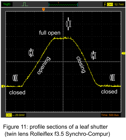
A first qualitative examination of the curve reveals the following:
- The curve has five distinct sections:
- shutter closed;
- opening;
- fully open;
- closing;
- shutter closed again.
- The fully open phase represents only a small part of the overall sequence.
- The opening phase is almost linear on this particular shutter.
- The closing phase is more rounded and slightly faster than the opening phase.
It should be noted that some of the electronic noise is caused by electromagnetic interference picked up by the cable connecting the tester to the oscilloscope probe.
Figure 12 provides a quantitative reading of the same graph.
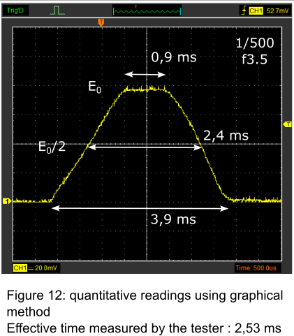
To measure a duration, it is simply necessary to count the number of divisions and multiply by the time represented by one division.
The following table summarizes the measurements obtained from this graph. The deviation in the right-hand column is relative to the effective exposure time measured by the tester.
| Measurement | Duration (ms) | Equivalent speed | Deviation (EV) |
|---|---|---|---|
| Shutter speed setting | 2.00 | 1/500 s | -0.33 |
| Effective exposure time (measured by the tester) | 2.53 | 1/396 s | – |
| Total duration | 3.9 | 1/256 s | +0.62 |
| Fully open duration | 0.9 | 1/1111 s | -1.5 |
| E0/2 duration | 2.4 | 1/417 s | -0.08 |
Interpretation
- There is a 1/3-stop difference between the nominal shutter speed and the effective shutter speed. This may seem significant, but it is quite typical of the highest speed of leaf shutters.
- Depending on the threshold used to define the beginning and end of the exposure, a timer-based measurement can give values ranging from 1/256 s to 1/1111 s, representing a difference of more than 2 EV.
- Measuring at the E0/2 threshold gives a result very close to the effective exposure time, with a deviation of only 0.08 EV. This small difference results from the opening profile being very close to a parallelogram, with sides that are symmetrical about their midpoint.
Measurements at Other Shutter Speed Settings
Figure 13 compares the effective exposure time with the total duration at nominal shutter speeds of 1/250 s and 1/125 s.
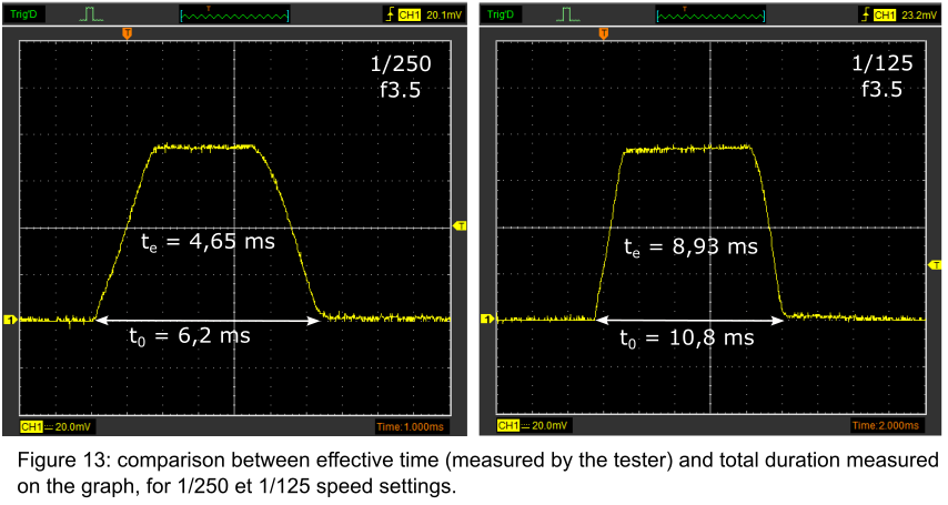
The measurements at the three shutter speed settings are summarized in the following table:
| Speed setting | 1/500 s | 1/250 s | 1/125 s |
|---|---|---|---|
| Effective exposure time | 2.53 ms | 4.65 ms | 8.93 ms |
| Total duration | 3.9 ms | 6.2 ms | 10.8 ms |
| Shutter efficiency | 65% | 75% | 83% |
The shutter efficiency is defined by the ration between the effective time and the total time. The higher the efficiency, the lower the transient phase contribute to the overal open time.
We can see that, in a leaf shutter, the contribution of the transient phases is particularly significant. Even two stops below the maximum speed, there is still a 17% difference between the total duration and the effective exposure time.
Measurements with a Stopped Down Aperture
Figure 14 shows the illuminance curve at a nominal shutter speed of 1/500 s, but with the aperture stopped down to f/5.6. Note that the illuminance scale has changed.
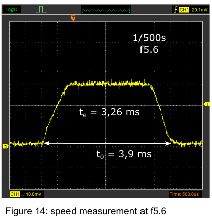
The following table compares the results with those obtained at f/3.5:
| f/3.5 | f/5.6 | |
|---|---|---|
| t0 | 3.9 ms | 3.9 ms |
| te | 2.53 ms | 3.26 ms |
| Effective speed (speed setting 1/500 s) | 1/395 s | 1/306 s |
| Measured illuminance | 76 mV | 30 mV |
Difference in aperture, f/3.5 to f/5.6: 1.36 stops
Difference in measured illuminance: 1.34 stops
The measurement at f/5.6 shows a truncated opening profile. Its total duration remains unchanged at 3.9 ms, but the curve is truncated at 30 mV instead of 76 mV at f/3.5. This is because only the central portion of the lens and shutter contributes to the illuminance.
Consequently, the effective exposure time is determined from the lower part of the opening profile, resulting in a slower effective shutter speed.
At f/5.6, there is therefore almost a 1 EV difference between the nominal shutter speed of 1/500 s and the effective shutter speed of approximately 1/300 s.
This experimentally demonstrates that the effective exposure time is not solely a mechanical property of the shutter. It also depends on the optical geometry in which the shutter is used.
This reduction in effective shutter speed when the aperture is stopped down at high shutter speeds is a phenomenon that should be taken into account when characterizing the shutter. By convention, shutter speed is therefore tested at full aperture.
It is worth noting that the measured illuminance difference of 1.34 EV corresponds almost exactly to the 1.36-stop difference in aperture on the camera.
This agreement provides an experimental verification of the linearity of the measurement chain: a known reduction in aperture produces a corresponding reduction in the measured signal.
Measurement with a Point Light Source
Figure 15 shows the illuminance curve obtained using a point light source instead of diffuse illumination, in this case, the integrated LED of the Baby Shutter Tester mkII.
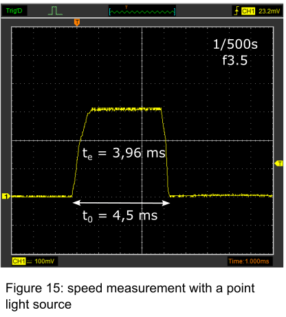
The illuminance curve has a truncated shape, even more pronounced than when the aperture is stopped down to f/5.6.
This can easily be explained by the fact that the point source illuminates only the central portion of the shutter. This produces an effect comparable to stopping down the aperture.
The measured effective exposure time is 3.96 ms, which is significantly different, by 0.7 EV, from the effective exposure time measured under the same conditions using diffuse light covering the entire lens: 2.4 ms.
The use of a light source that is not diffuse and uniform is therefore clearly a source of measurement error.
Comparison of Several Shutter Models
Figure 16 compares the opening profiles of several shutter models at their maximum speeds:
- Rolleiflex Synchro-Compur f/3.5 (~1965);
- Lubitel 166, T-22 f/4.5 (~1990?);
- Kodak 620 f/6.3 (~1950).
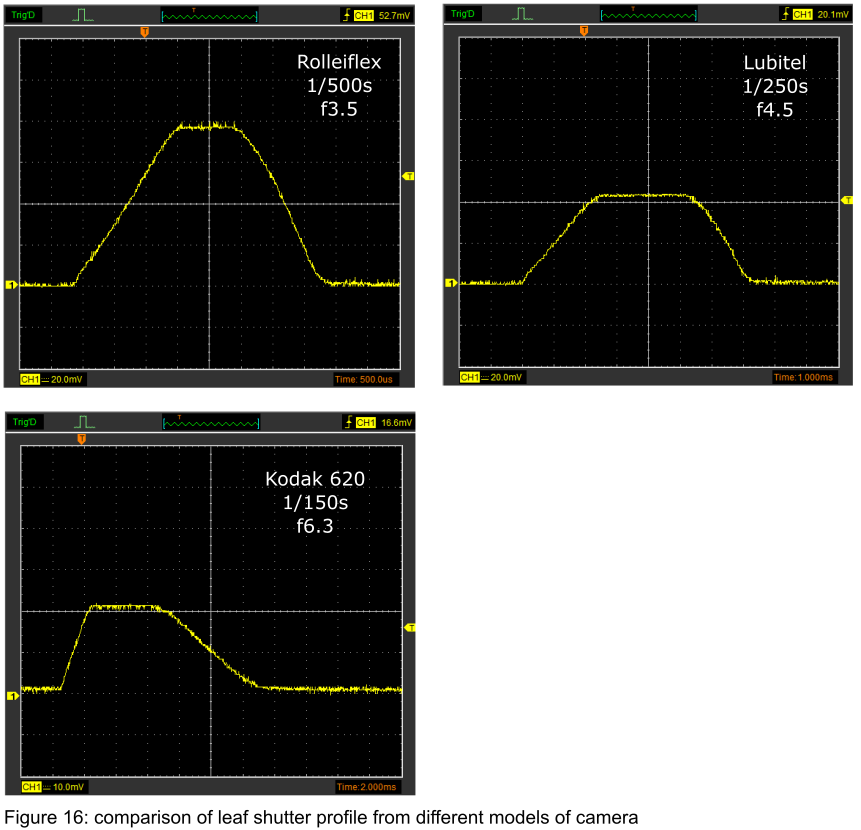
The curves of these different shutters, despite their very different ages and levels of quality, show strong similarities:
- very pronounced transient phases;
- a shape close to a parallelogram.
The observations made on the Rolleiflex shutter therefore appear to be applicable to the other leaf-shutter models tested.
Conclusions
The different measurements presented in this article lead to the following conclusions:
- Leaf shutters have opening profiles with very pronounced transient phases.
- Timer-based shutter-speed measurements can differ by more than 1 EV from the effective exposure time, depending on the threshold used.
- Timer-based measurement at the E0/2 threshold produces a result very close to the effective exposure time.
- This threshold must nevertheless be recalibrated for each different shutter if its characteristics (aperture, associated focal length, etc.) are different.
- Integration-based measurement requires no calibration procedure because it directly provides the effective exposure time by definition (see the previous article).
- A diffuse light source, uniform over the entire shutter aperture, is required to obtain reliable results.
- The effective shutter speed decreases when the aperture is stopped down, although shutter speed is conventionally tested at full aperture.
- The voltage measured at different aperture settings indicates very good linearity in the Baby Shutter Tester mkII’s electronic circuits.

 English
  French
Leave a Reply